Getting started

VARcheck visualises the fit of vector autoregressive (VAR) models through a multi-panel diagnostic grid. The package does not fit models. Instead, it takes the outputs of your existing workflow and turns them into a structured plot.

Setup

library(VARcheck)
set.seed(35032)

Creating a `var_data` object

new_var_data() takes three required inputs (empirical data, model predictions, and residuals), each as a T × p numeric matrix (time points × variables). Simulated data for posterior predictive checks is optional but enables the rightmost column of the diagnostic grid.

The example below simulates a simple two-variable VAR(1) process directly, without any modelling package.

# Simulate a VAR(1) process
T  <- 150
p  <- 4
phi <- matrix(c(0.5, 0.1, 0.0, 0.0,
                0.2, 0.4, 0.0, 0.1,
                0.0, 0.0, 0.6, 0.0,
                0.1, 0.0, 0.2, 0.3), nrow = p, byrow = TRUE)

emp <- matrix(0, T, p)
for (t in 2:T) {
  emp[t, ] <- phi %*% emp[t - 1, ] + rnorm(p, sd = 0.5)
}

# Fit a simple lag-1 linear model per variable (stand-in for a real VAR fit)
pred <- matrix(NA, T, p)
res  <- matrix(NA, T, p)
for (j in seq_len(p)) {
  fit        <- lm(emp[-1, j] ~ emp[-T, j])
  pred[-1, j] <- predict(fit)
  res[-1, j]  <- residuals(fit)
}

# Simulate from the fitted model for the posterior predictive check
sim <- matrix(0, T, p)
for (t in 2:T) {
  sim[t, ] <- phi %*% sim[t - 1, ] + rnorm(p, sd = 0.5)
}

vd <- new_var_data(
  empirical  = emp,
  predicted  = pred,
  residuals  = res,
  simulated  = sim,
  var_names  = c("Mood", "Energy", "Fatigue", "Anxiety")
)

vd
#> <var_data>
#>   Subjects  : 1 
#>   Variables : 4 ( Mood, Energy, Fatigue, Anxiety )
#>   Timepoints  : 150 
#>   Components: empirical, predicted, residuals, simulated

The diagnostic grid

plot_var_check() returns a patchwork object, so it can be printed, saved with ggplot2::ggsave(), or combined with other plots.

plot_var_check(vd)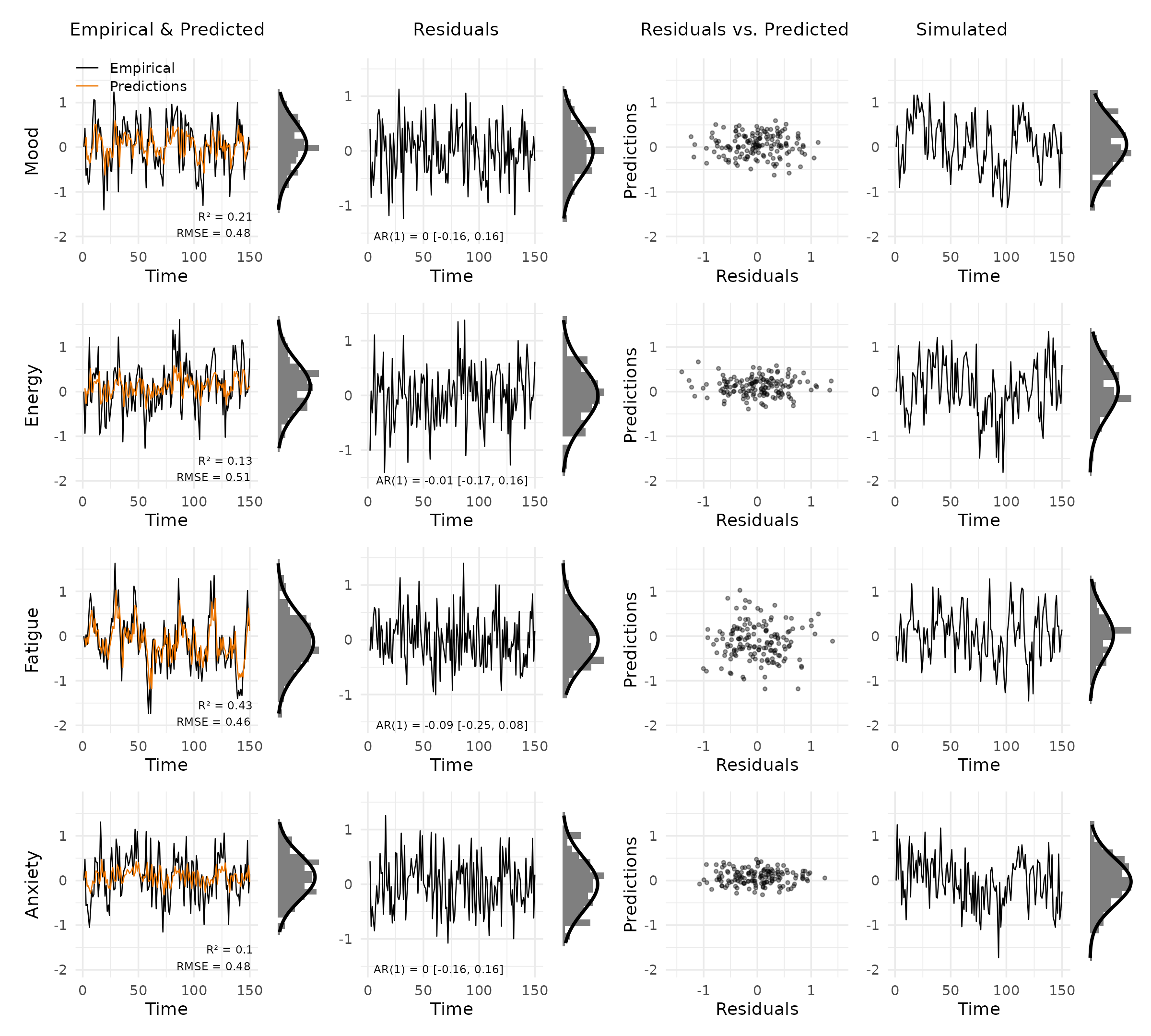

Each row shows one variable. The columns are:

Empirical & Predicted: observed values (black) against predictions (orange), with R² and RMSE in the bottom right. The small panel to the right is a marginal histogram with a Gaussian overlay.
Residuals: residuals over time, annotated with the AR(1) coefficient and 95% CI to flag autocorrelation.
Residuals vs. Predicted: scatter of residuals against predictions. A clear pattern here signals model misspecification.
Simulated: data simulated from the fitted model, for visual comparison with the empirical series.

Selecting variables and panels

Show only a subset of variables by name or index:

plot_var_check(vd, vars = c("Mood", "Fatigue"))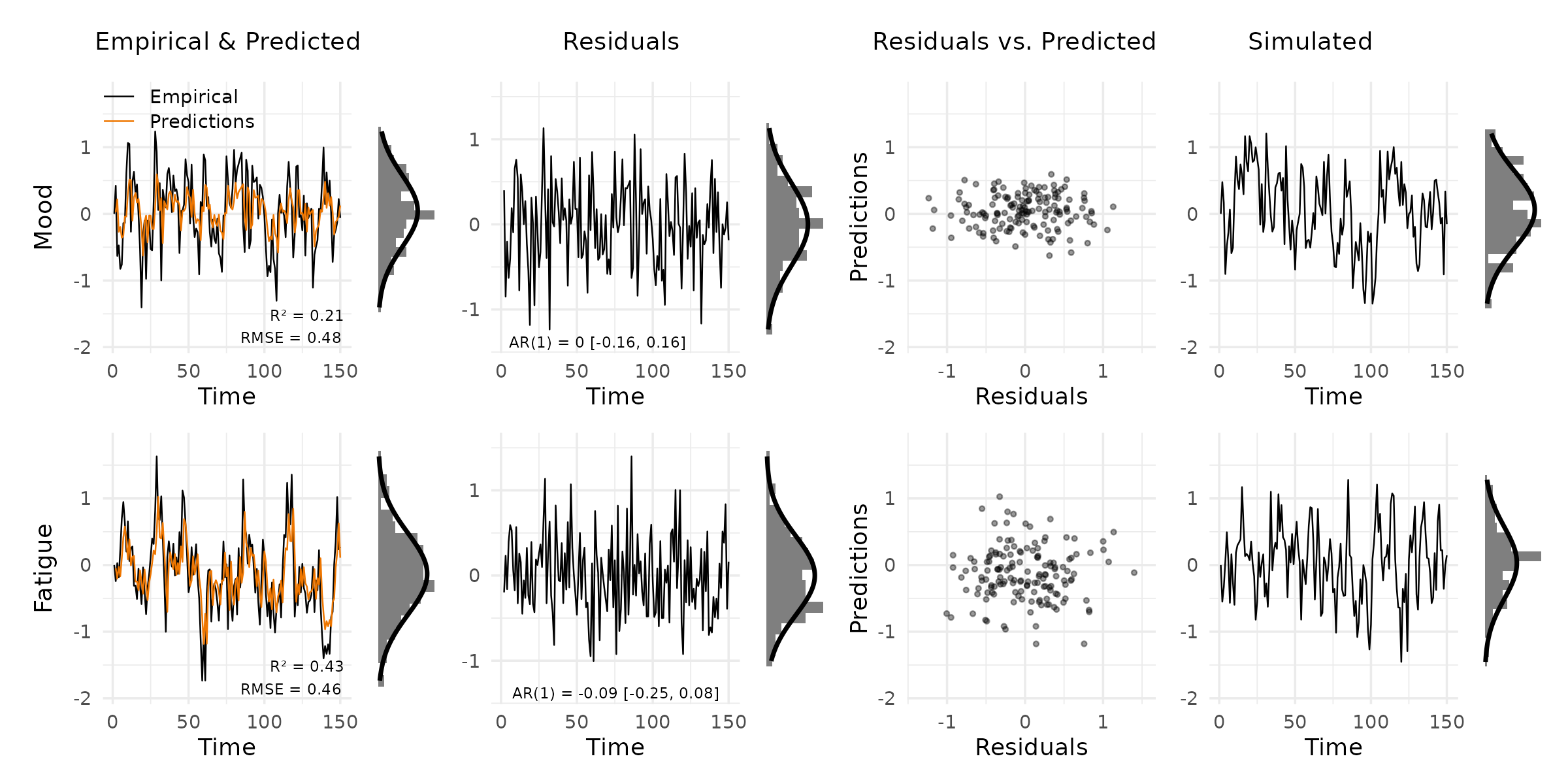

Drop columns you do not need. The layout adjusts automatically:

plot_var_check(vd, panels = c("data", "residuals"))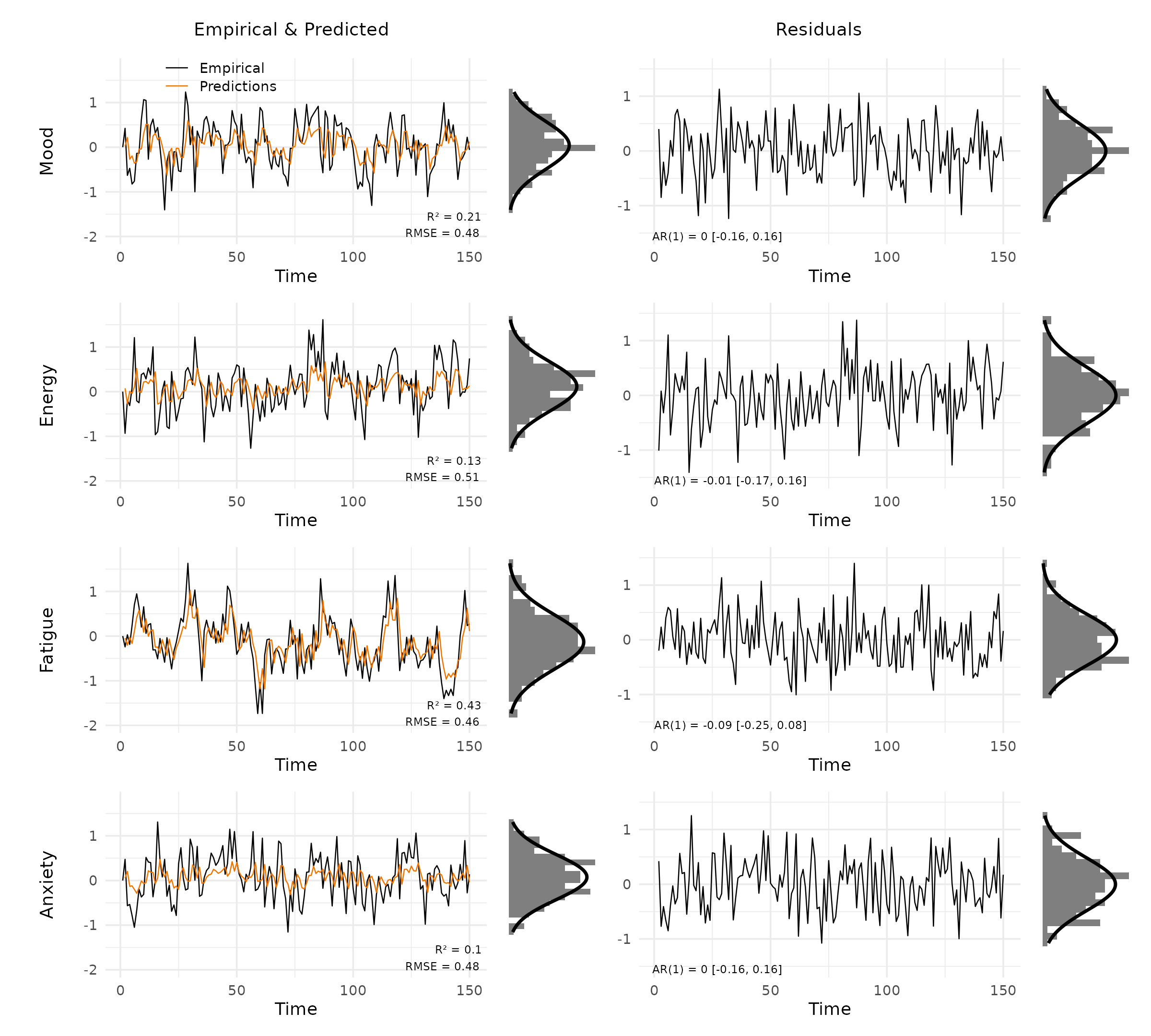

Multiple subjects

When data comes from multiple people, pass a list of matrices (one per subject) to new_var_data(). Use the subject argument to choose which one to plot.

emp2  <- emp + matrix(rnorm(T * p, sd = 0.2), T, p)
pred2 <- pred + matrix(rnorm(T * p, sd = 0.1), T, p)
res2  <- emp2 - pred2

vd_multi <- new_var_data(
  empirical = list(emp, emp2),
  predicted = list(pred, pred2),
  residuals = list(res, res2),
  simulated = list(sim, sim),
  var_names = c("Mood", "Energy", "Fatigue", "Anxiety")
)

plot_var_check(vd_multi, subject = 2)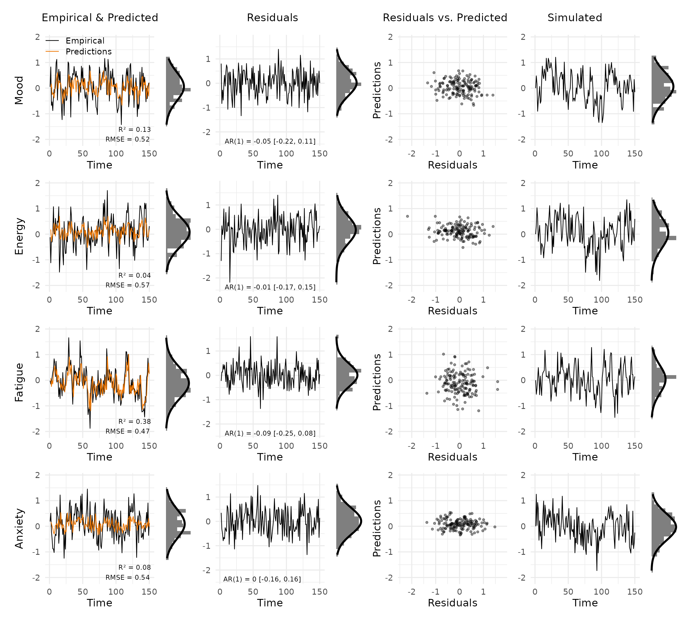

Customisation

Colours: pass a named list with empirical and/or predicted keys. Unspecified keys retain their defaults.

plot_var_check(vd, colors = list(predicted = "steelblue4"))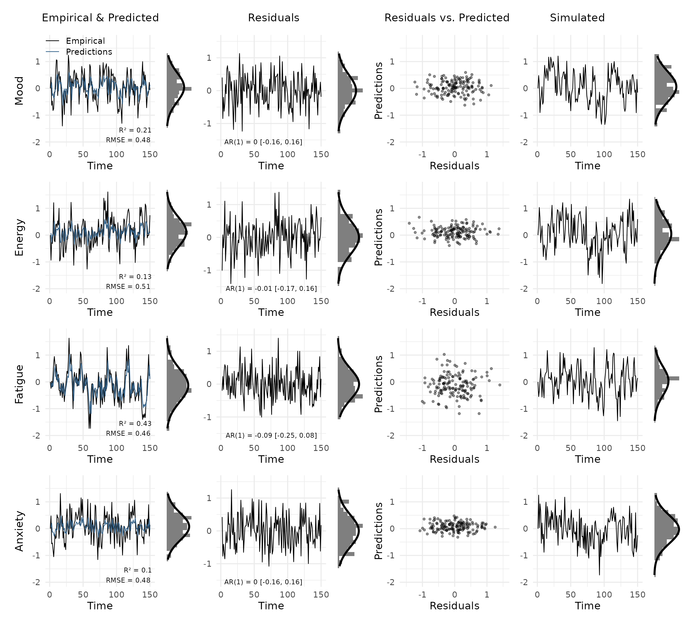

Theme: the default is theme_varcheck(). Add any ggplot2::theme() call on top of it via the theme argument.

plot_var_check(
  vd,
  theme = ggplot2::theme(
    text      = ggplot2::element_text(size = 9, family = "sans"),
    panel.grid.minor = ggplot2::element_blank()
  )
)

Shared y-limits: by default, limits are computed across all selected variables. Override them when comparing across subjects or model variants.

plot_var_check(vd, ylim_data = c(-3, 3), ylim_res = c(-2, 2))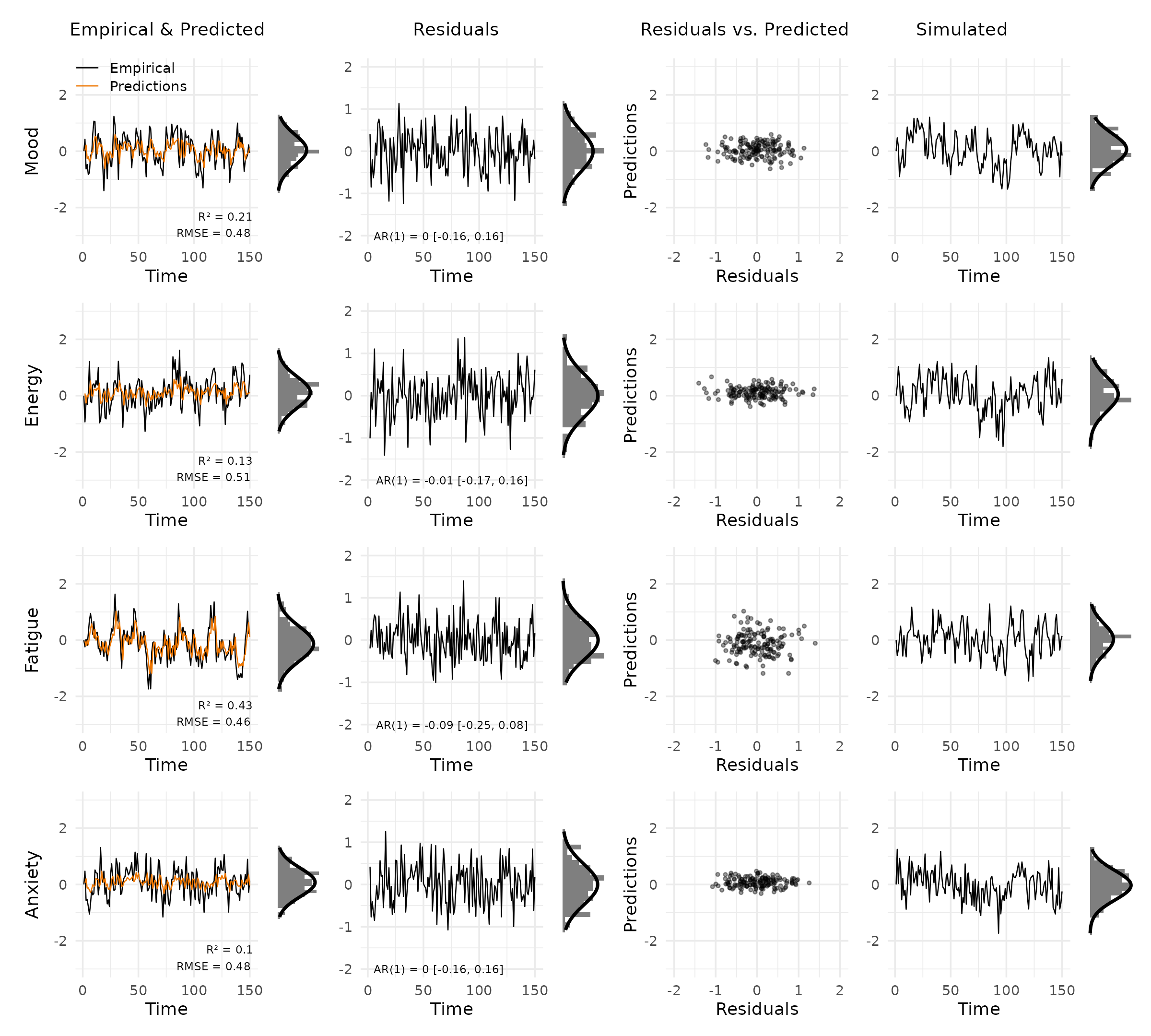

Using mlVAR outputs

If you fit a model with mlVAR, the residuals() and predict() methods return per-subject data frames. The code below shows how to assemble them into a var_data object. new_var_data() requires numeric matrices, so call as.matrix() on each data frame.

Assume you have already run:

library(mlVAR)

mlVAR_out <- mlVAR(data, vars = c("A", "B", "C", "D"),
                   idvar = "id", lags = 1,
                   dayvar = "day", beepvar = "beep")

pred_df <- predict(mlVAR_out)
res_df  <- residuals(mlVAR_out)
sim_out <- mlVAR:::resimulate(mlVAR_out, keep_missing = TRUE,
                              variance = "empirical")

Single subject

i <- 1  # subject index
unique_ids <- unique(data$id)

check_df <- new_var_data(
  empirical = as.matrix(data[data$id == unique_ids[i], vars]),
  predicted = as.matrix(pred_df[pred_df$id == unique_ids[i], vars]),
  residuals = as.matrix(res_df[res_df$id == unique_ids[i], vars]),
  simulated = as.matrix(sim_out[sim_out$id == unique_ids[i], vars])
)

plot_var_check(check_df)

All subjects

Pass a list of matrices (one per subject) to plot any individual later with subject = i.

vars     <- c("A", "B", "C", "D")
n_subj   <- length(unique_ids)

check_df_all <- new_var_data(
  empirical = lapply(unique_ids, \(id) as.matrix(data[data$id == id, vars])),
  predicted = lapply(unique_ids, \(id) as.matrix(pred_df[pred_df$id == id, vars])),
  residuals = lapply(unique_ids, \(id) as.matrix(res_df[res_df$id == id, vars])),
  simulated = lapply(unique_ids, \(id) as.matrix(sim_out[sim_out$id == id, vars]))
)

plot_var_check(check_df_all, subject = 3)