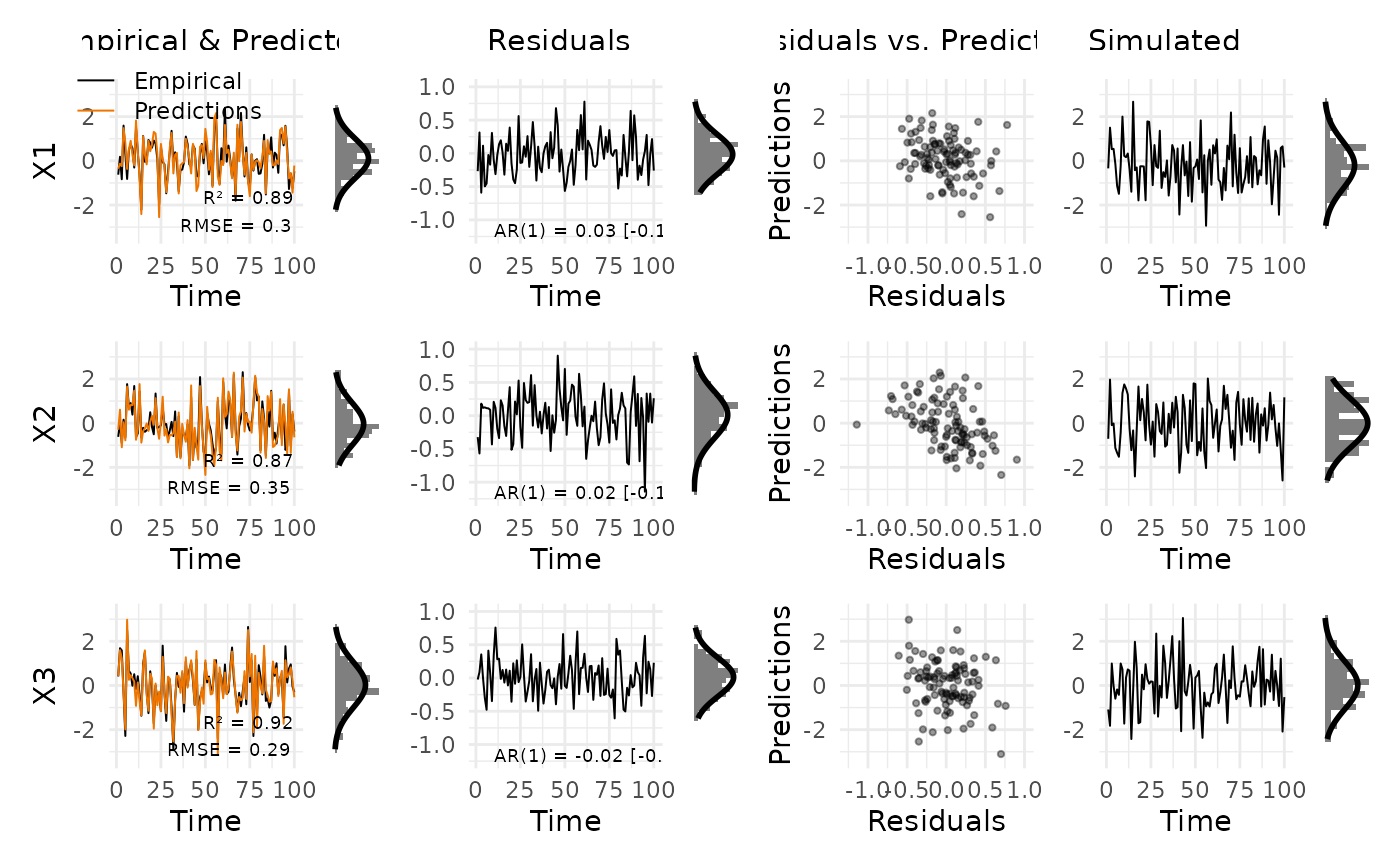
Plot VAR model diagnostics — plot_var

Creates a multi-panel diagnostic grid for a fitted VAR model. Each row corresponds to one variable; columns show (a) empirical data vs. predictions, (b) residuals over time, (c) residuals vs. predictions scatter, and (d) data simulated from the estimated model. Each time-series panel is accompanied by a marginal histogram with a Gaussian overlay.

Usage

plot_var_check(
  data,
  subject = 1,
  vars = NULL,
  panels = c("data", "residuals", "scatter", "simulated"),
  colors = list(),
  theme = NULL,
  ylim_data = NULL,
  ylim_res = NULL
)

Arguments

data: A `var_data` object created with [new_var_data()].
subject: Integer. Index of the subject to plot. Defaults to `1`.
vars: Character or integer vector selecting variables to include. Defaults to all variables.
panels: Character vector controlling which columns are shown. Any subset of `c("data", "residuals", "scatter", "simulated")`, in that order. Defaults to all four.
colors: Named list controlling line colours. Recognised elements: `empirical` (default `"black"`) and `predicted` (default `"darkorange2"`). Partial lists are merged with the defaults.
theme: A `ggplot2::theme()` object added on top of [theme_varcheck()]. Use this to override individual theme elements.
ylim_data: Numeric vector of length 2. Shared y-limits for the data-scale panels (empirical/predicted/simulated). Auto-computed from the data if `NULL`.
ylim_res: Numeric vector of length 2. Shared y-limits for the residual panels. Auto-computed from the residuals if `NULL`.

Value

A `patchwork` object.

Examples

set.seed(1)
emp <- matrix(rnorm(300), nrow = 100, ncol = 3)
pred <- emp + matrix(rnorm(300, sd = 0.3), 100, 3)
res <- emp - pred
sim <- matrix(rnorm(300), 100, 3)
vd <- new_var_data(emp, pred, res, sim, var_names = c("X1", "X2", "X3"))
# \donttest{
plot_var_check(vd)

# }